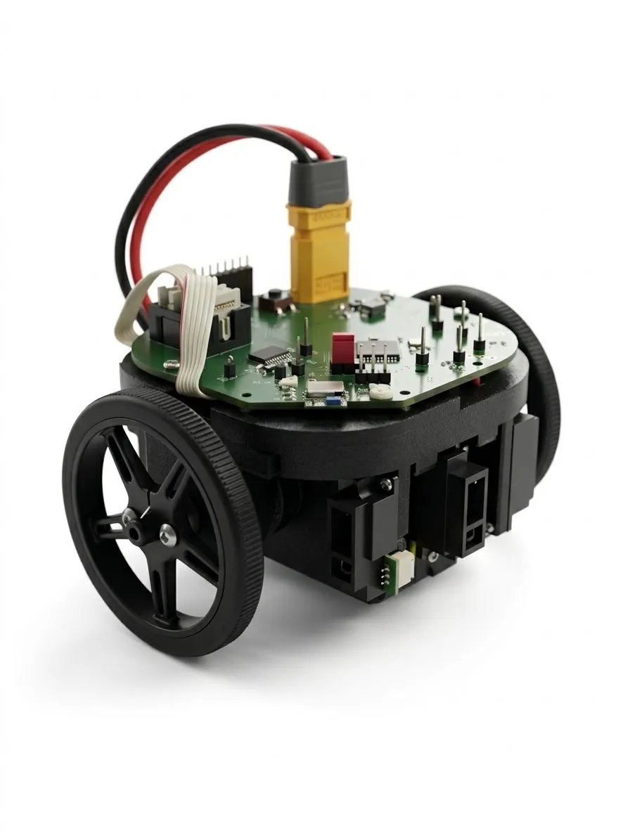
Jerry is a small autonomous robot. Placed in a maze it has never seen before, it finds its way to the center on its own and then races there as fast as it can. Over one semester at TUM, our team of four designed, built and programmed Jerry from scratch: from the schematic and the PCB, over a 3D-printed chassis, to the firmware that explores and solves the maze.
This post summarizes the project: the main design decisions, the problems we ran into and what we learned from them.
The challenge
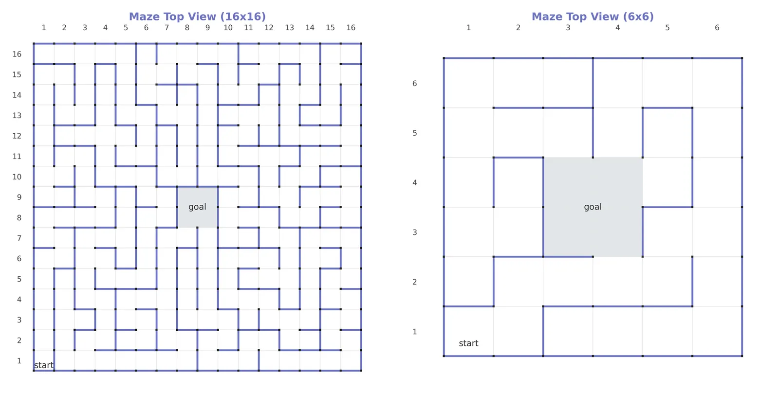
In the official competition, a micromouse has to solve a 16 × 16 maze. It starts in a dead end in one corner and has to reach the 2 × 2 goal area in the center. The robot knows the dimensions of the maze, but not its layout. A run therefore has three phases: explore the maze, return to the start, and finally race to the center on the shortest path.
For our lab, we used a smaller 6 × 6 maze. It is smaller, but poses the same fundamental problems: detect walls reliably, always know where you are, and never touch a wall while doing so.
We defined the following goals:
- Sensing: reliable wall detection with calibrated infrared sensors and precise wheel odometry from the motor encoders
- Motion: closed-loop control to drive centered between the walls, plus in-place 90° and 180° turns
- Mapping: a memory-efficient maze representation on the microcontroller, autonomous exploration and flood-fill path planning
- Validation: reliable runs in the physical lab maze, with code that scales to the 16 × 16 format
The building blocks
The microcontroller, the motors and the battery were given by the course. We selected and designed everything else ourselves.
| Component | Choice | Notes |
|---|---|---|
| Microcontroller | dsPIC33FJ64MC804 | 16-bit DSC with 40 MIPS, 16 KB RAM and dedicated ADC, PWM and encoder peripherals |
| Motors | 2× Faulhaber 2619S006SR | 6 V coreless DC motors with 33:1 gearbox and integrated encoders |
| Battery | 2S LiPo (7.4 V) | Powers the motors directly and the logic through regulators |
| Distance sensors | 3× Sharp GP2Y0A51SK0F | Analog IR sensors for 2–15 cm, fast and compact |
| Motor driver | TB6612FNG dual H-bridge | Drives both motors from one IC, 1.2 A per channel |
| Communication | RN4871 Bluetooth LE + UART | Wireless debugging while the mouse is driving |
| Drive | Differential drive + felt gliders | Turns in place; no casters needed on the smooth maze floor |
A rough estimate confirmed that the motors are strong enough: accelerating a 0.5 kg robot at 1.5 m/s² with 60 mm wheels needs about 11 mNm per wheel, while the geared motors deliver around 30 mNm continuously.
Designing the PCB
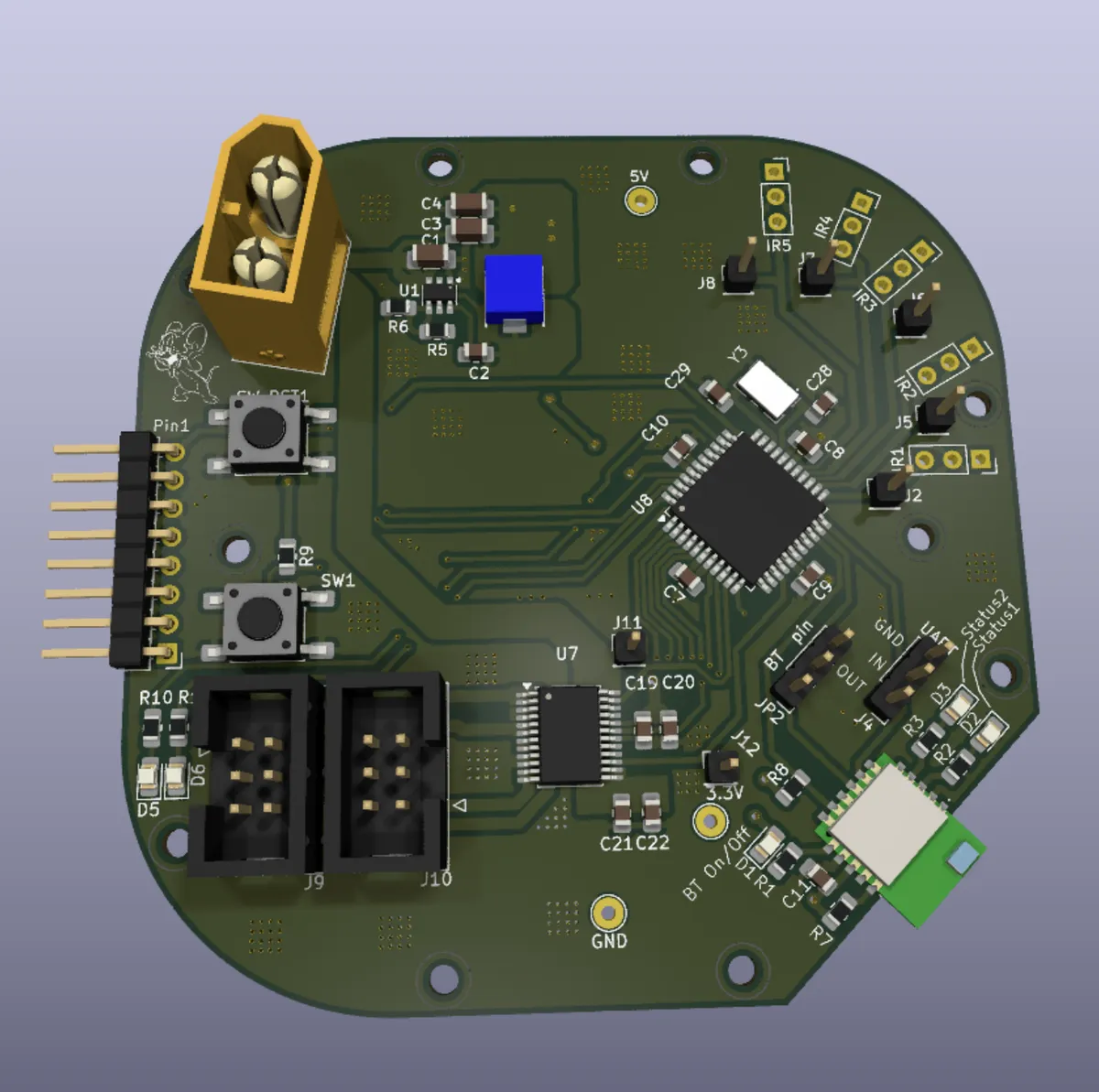
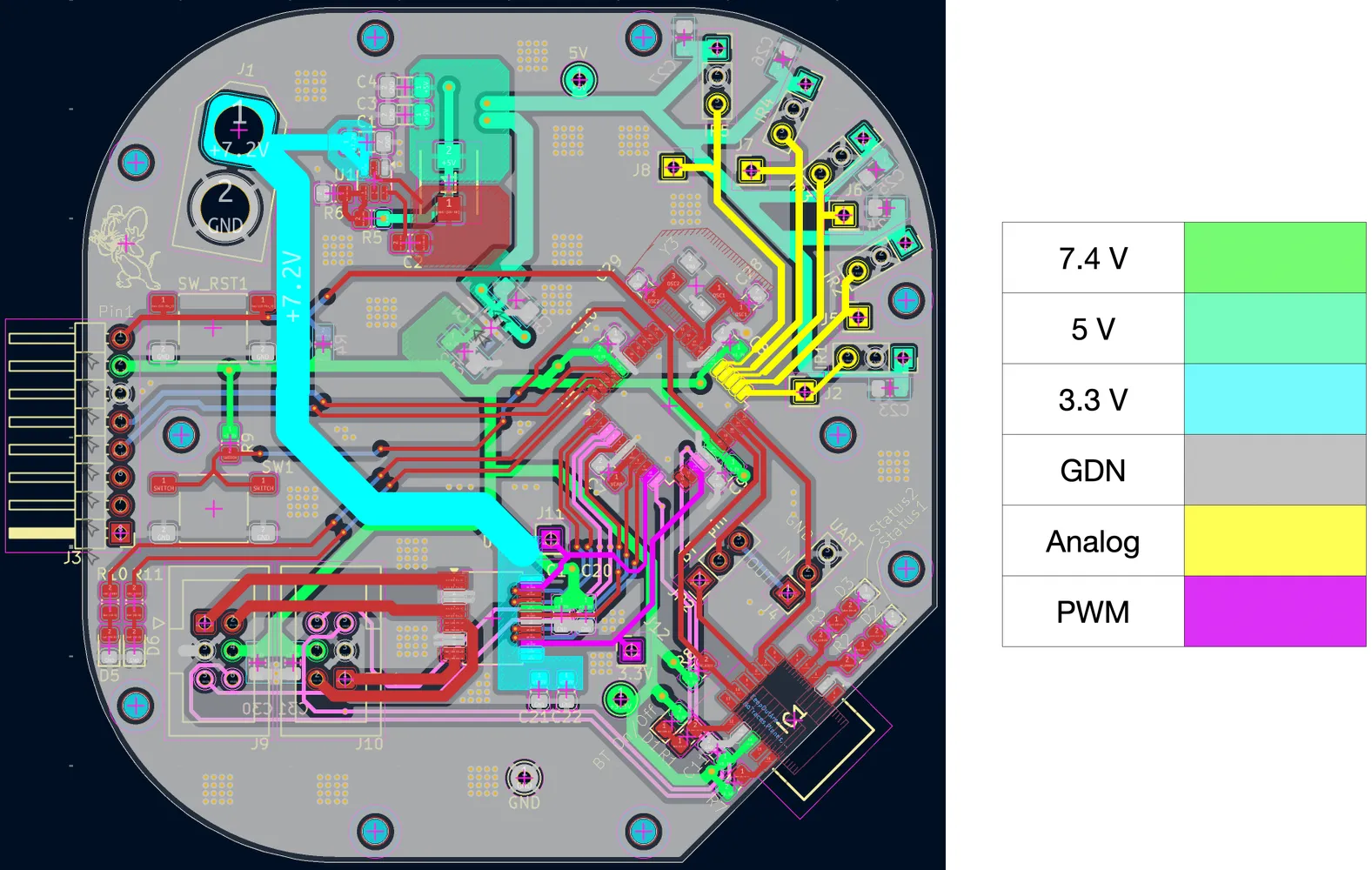
We designed the board in KiCad. For the layout, we followed a few simple rules: keep the power supply close to the main consumers (the H-bridge and motors), keep traces short, avoid unnecessary crossings and keep the noisy PWM lines away from the sensitive analog sensor signals.
The microcontroller sits in the center with sensors, communication and peripherals arranged around it. We added an 8 MHz crystal, which the internal PLL multiplies to an 80 MHz oscillator frequency (40 MHz instruction clock), a programming header, a start and a reset button, and connectors for two optional diagonal sensors. For the Bluetooth module, we cut away a corner of the board so that there is no copper below its antenna.
Power: a two-stage cascade
Jerry runs on a single 2S LiPo battery (7.4 V nominal, up to 8.4 V fully charged), but the electronics need 5 V and 3.3 V. Instead of deriving both rails from the battery in parallel, we cascade them:
- Motors are powered directly from the battery through the H-bridge. Their current spikes, e.g. when changing direction, therefore never reach the logic rails.
- 5 V for the sensors comes from a synchronous buck converter (AP62300, up to 3 A). A linear regulator would have turned about 2.4 W into heat at 1 A.
- 3.3 V for the microcontroller, Bluetooth module and encoders comes from a low-dropout regulator (TLV757P) fed by the 5 V rail. It adds no switching noise of its own and suppresses the ripple of the buck converter (46 dB PSRR at 100 kHz). This keeps the supply of the microcontroller and its ADC inputs clean.
Even in the worst case, the 5 V rail only has to supply around 450 mA, well below the 3 A the converter can deliver.
Motors and PWM
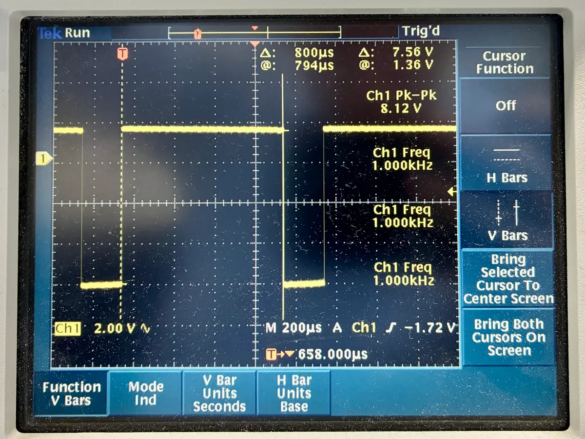
The motors are rated for 6 V, the battery delivers 7.4 V. Rather than adding another regulator, we cap the PWM duty cycle at 6 V / 7.4 V ≈ 80 %, which keeps the average motor voltage close to its rating. The PWM runs at 1 kHz.
Putting Jerry on a diet: the casing
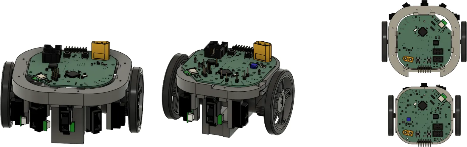
Many micromice mount their motors directly onto the PCB. We decided against that to keep mechanical stress off the board and designed a 3D-printed casing instead. It holds the motors, sensors and battery and carries the PCB on top.
The first version started as a simple frame and gradually gained sensor mounts, motor cutouts, mounts for two diagonal sensors and a cutout for the programmer. Originally, the battery was supposed to sit on top. That would have raised the center of gravity and blocked access to the buttons and the programming header, so we flipped the design: battery at the bottom, PCB on top.

After the first test runs, we noticed that this casing was too wide for tight corners. So we put Jerry on a diet: the second casing is much narrower, drops the two diagonal sensors in favor of a longer measuring range for the side sensors, and reduces the wheel-to-wheel distance from 130 mm to 103 mm.
From parts to a robot
We already learned a few things while ordering the parts:
- Order parts that are well in stock. A single part with low availability delayed our shipment by a week, which then ran into the holiday season and cost us another two weeks.
- Order spares. Most components cost only a few cents, so ordering at least one extra of each covers lost or damaged parts at almost no cost.
- Order alternatives for parts that might hit their thermal or electrical limits. We ordered two footprint-compatible voltage regulators, one with and one without a thermal pad.
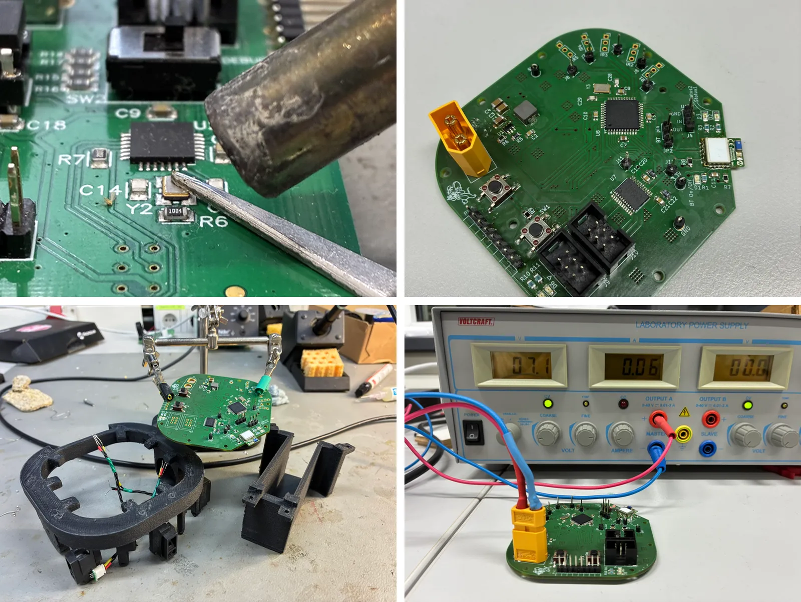
We soldered with lead-free solder at about 350 °C, working from the center of the board outwards and from small to large components. Parts with pads underneath, like the crystal oscillator or the regulator's thermal pad, were soldered with a hot air gun. Afterwards, we mounted the sensors in the casing and twisted their power, ground and signal wires to reduce interference.
For the first power-up, we used a lab power supply with a 0.6 A current limit, so that a short circuit could not destroy anything. That worked well until we enabled the PLL: the higher clock rate drew more current than the limit allowed, and Jerry started rebooting seemingly at random until we noticed that the power supply was throttling him.
One more lesson: solder the XT60 battery connector with its counterpart plugged in. We didn't, the nylon inside got too hot, and the pins ended up misaligned.
Firmware
The firmware is written in C and built with MPLAB X and the XC16 compiler. It is split into clearly separated layers: a hardware abstraction layer at the bottom, motion control in the middle and maze solving on top. The maze solver only asks for things like "drive three cells forward" or "turn left" and leaves the execution to the motion controller. This way, the same motion primitives are reused for exploration, the return to the start and the final speed run.
Timers instead of an RTOS
Instead of a real-time operating system, all periodic work is driven by three hardware timers:
| Timer | Period | Task |
|---|---|---|
| Timer 1 | 10 ms | Edge detection of the start button |
| Timer 2 | 400 ms | Process incoming Bluetooth commands |
| Timer 3 | 10 ms | Motion control and navigation step |
To keep the interrupt routines short, the timers mostly just set a flag and the actual work happens in the main loop. A small helper, initTimerInMS(id, ms), picks the smallest prescaler that fits the requested period into the 16-bit timer.
Sensing walls
Three Sharp infrared sensors look to the left, to the front and to the right. They output an analog voltage that depends on the distance to the wall. The ADC scans all three channels in 12-bit mode, and a DMA channel copies every result straight into memory, so the rest of the code reads the latest value with a simple array access and without any CPU overhead. At roughly 10 µs per full scan, this is far faster than the sensors themselves, which only update every 16.5 ms.
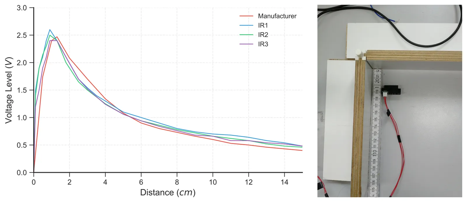
We calibrated each sensor against the actual maze walls. This was more important than we expected, because the sensors deviate noticeably from the datasheet curve and from each other. In early tests, Jerry constantly drifted to the right because we used a single calibration table for all sensors. Individual tables for each sensor fixed the problem.
Encoders and odometry
Both motor encoders are read by the microcontroller's quadrature encoder interfaces in 4× mode. With 16 pulses per motor revolution, 4× decoding and the 33:1 gearbox, one wheel revolution yields 16 · 4 · 33 = 2112 ticks, which is about 11.2 ticks per millimeter with 60 mm wheels. Interpreting the difference between two readings of the 16-bit hardware counter as a signed value correctly handles over- and underflows.
Bluetooth for debugging
A cable works while the robot sits on the desk, but not once it drives through the maze. So we added an RN4871 Bluetooth Low Energy module in transparent UART mode: for the firmware, the wireless link behaves like a serial cable. Every message is wrapped in angle brackets (e.g. <MAP>), which makes it easy to discard incomplete or garbled input.
On the PC side, a small Python console based on the Bleak library connects to Jerry. Over time, the command set grew into a full tuning interface: start the mapping or the speed run, drive or turn on command, print sensor values and encoder ticks, adjust geometry and overshoot parameters at runtime, and print the current maze as ASCII art. Being able to tune parameters without reflashing the firmware saved us a lot of time.
Driving straight: motion control
Driving is based on simple geometry. The maze cells measure 168 mm on the inside plus a 13 mm wall, so driving n cells means driving n · 181 mm worth of encoder ticks. For a turn, each wheel travels along a circle whose diameter is the 103 mm wheel-to-wheel distance.
In practice, the wheels and motors are never perfectly identical, so a controller has to keep Jerry centered between the walls. We use a PD controller on the difference between the measured and the expected side distances. An additional motorTrim term compensates for a constant difference between the two motors and is slowly adapted while driving:
int E  = ((dLeftIs - dLeftShould) - (dRightIs - dRightShould)) / 2;
int dE = E - lastE;

float pTerm = KP * (float)E;
float dTerm = KD * (float)dE;
int totalCorrection = (int)lroundf(pTerm + dTerm + motorTrim);

int speedMotorA = baseSpeed - totalCorrection;
int speedMotorB = baseSpeed + totalCorrection;
lastE = E;
Tuning the controller
We tuned the controller in the usual way: start with KD = 0 and increase KP until the robot noticeably oscillates between the walls. If KP is too small, Jerry reacts too slowly and clips walls; if it is too large, he oversteers. Then KD is increased to damp the oscillation until the mouse settles smoothly in the center.
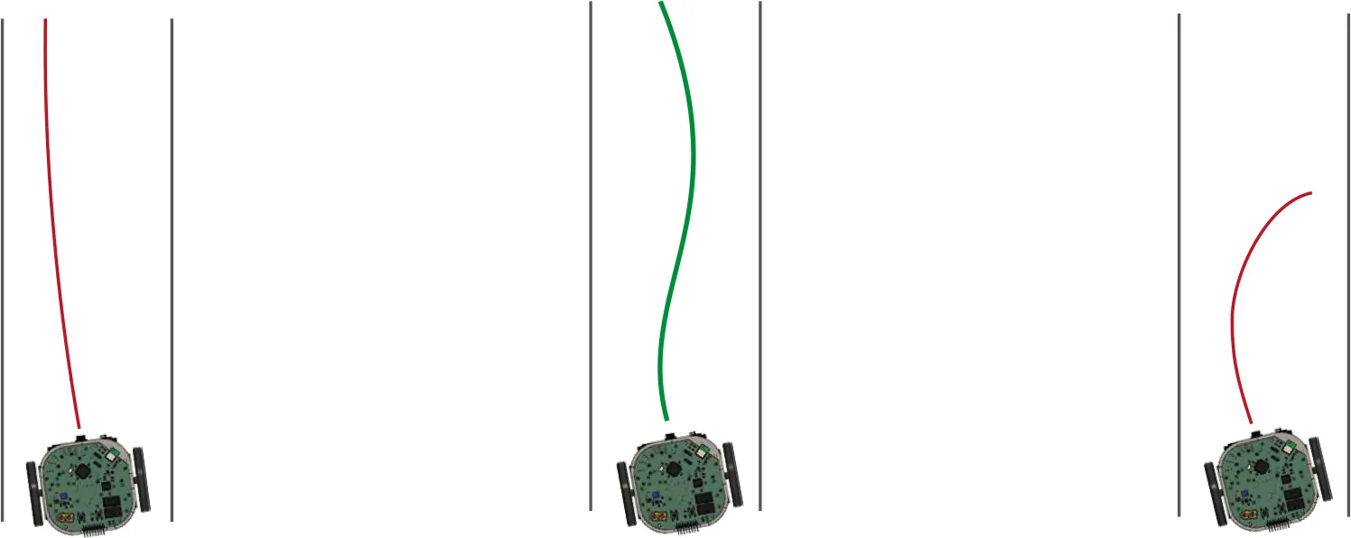
After a series of full maze runs around the first stable values, we settled on KP = 0.25 and KD = 0.4.
Our biggest mistake was to tune on a straight section only, planning to handle corners later. Values that work well on a straight turned out to fail at junctions and corners, where one or both side walls are missing. It worked much better to tune on a complete test maze, start slow, and increase the speed step by step while re-checking stability.
Turns had a separate problem: they overshot their target angle, and not proportionally to the angle, so a constant correction factor was not enough. Calculating the tick counts from the wheel geometry and adding an overshoot compensation that can be tuned via Bluetooth solved this.
Solving the maze
Keeping a map
Each cell can have a wall on any of its four sides, so 4 bits per cell are enough. Jerry keeps a 2D array of wall bitmasks, a separate grid of visited cells and his current pose:
// bitmask: 1 = N, 2 = E, 4 = S, 8 = W
static int walls[MAZE_SIZE][MAZE_SIZE];
static int visit[MAZE_SIZE][MAZE_SIZE];

typedef struct {
    unsigned int x;
    unsigned int y;
    Direction heading;
} Pose;
Walls are only measured while Jerry stands still in the center of a cell, where the sensor readings are most reliable. The relative readings (left, front, right) are converted to absolute directions using the current heading. Since every wall belongs to two cells, it is stored in the neighboring cell as well.
Exploring
During exploration, Jerry does not need to be fast. He runs a breadth-first search (BFS) from his current position to find the nearest unvisited cell, treating walls he hasn't seen yet as open. He then drives there cell by cell, recording walls and marking cells as visited. If an unexpected wall shows up in front of him, the planned path is no longer valid, so he discards it and plans again with the updated map. Once every reachable cell has been visited, he plans a path back to the start.
Racing
With the complete map, the classic flood-fill algorithm computes the shortest path: the four goal cells get the distance 0, their reachable neighbors 1, and so on. Jerry then simply follows decreasing values until he reaches 0.
+---+---+---+---+---+---+
| 4   5 | 5   4   3 | 4 |
+   +   +   +   +   +   +
| 3 | 6   6 | 5 | 2   3 |
+   +---+---+---+   +---+
| 2   1   0   0   1   2 |
+   +---+   +   +---+   +
| 3   4 | 0   0 | 4   3 |
+---+   +---+---+   +---+
| 6   5 | 7   6   5   6 |
+   +   +---+---+   +---+
| 7 | 6   7   7   6   7 |
+---+---+---+---+---+---+
Stopping and starting again at every cell wastes a lot of time. So before driving, consecutive cells in a straight line are merged into a single "drive n cells forward" command. This made the cell traversal 41.6 % faster and saved 0.26 s per cell on a five-cell straight.
Results
We tested Jerry in a number of different maze configurations. In every one of them, he explored and mapped all reachable cells correctly, returned to the start and drove to the goal on the shortest known path. The ASCII maps he sent over Bluetooth made it easy to compare his internal model with reality.
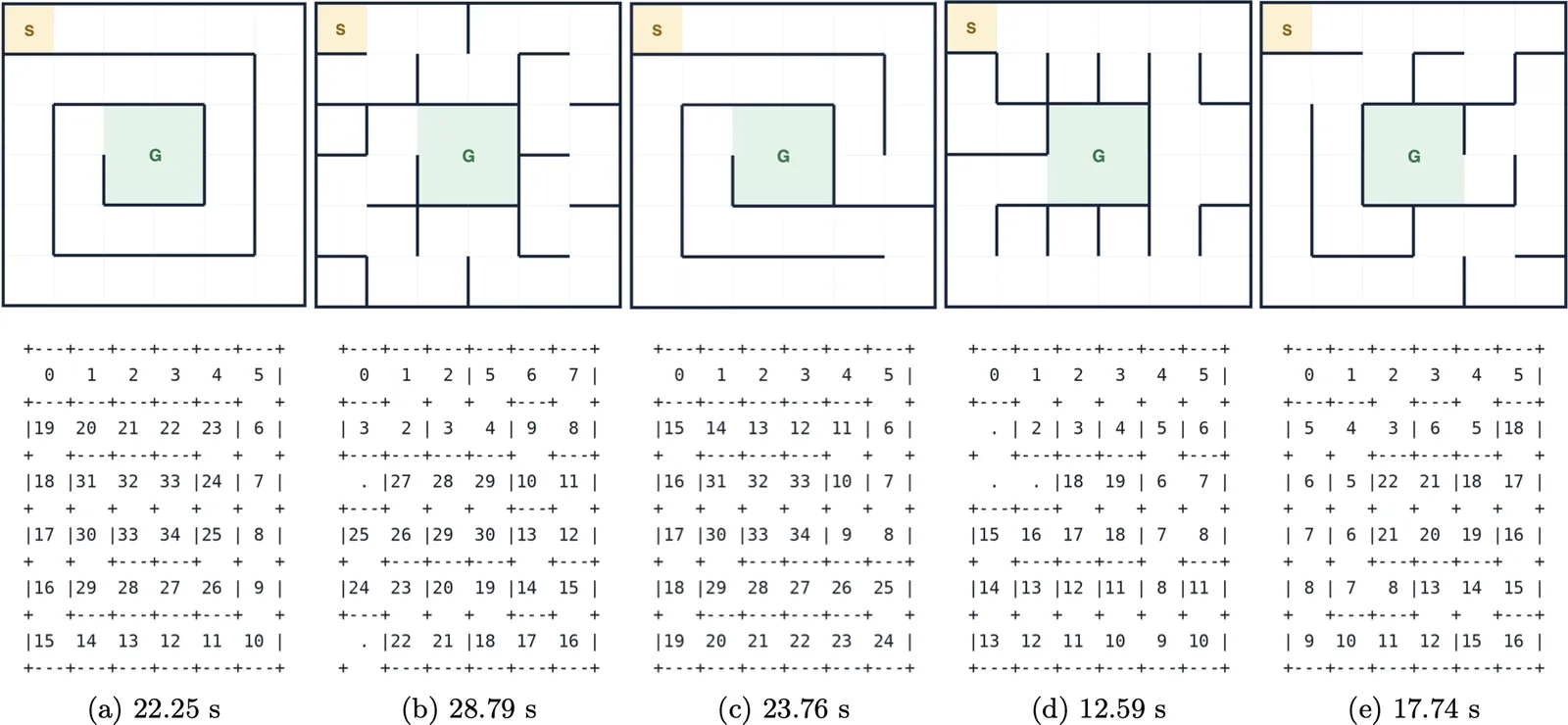
The maze size is a compile-time parameter and the algorithms don't depend on it. A full 16 × 16 maze needs only a few kilobytes, which fits easily into the 16 KB of RAM. Only the fixed buffer sizes for the path and the BFS queue would have to grow before Jerry can take on a competition maze.
Lessons learned
- Build incrementally. First each component on its own, then single moves and turns, and only then the full mapping. Testing many new parts at once makes errors very hard to find.
- Measure, don't trust the datasheet. Sensors, motors and turns all deviated noticeably from their nominal values. Wherever possible, we used measured values instead.
- Invest in debugging tools early. The Bluetooth command interface and the ASCII maze printouts helped us find most of our bugs.
- C doesn't check array bounds. An inverted condition in the flood-fill neighbor check read outside of the maze array. The program did not crash, but read random values and occasionally made wrong driving decisions. Routing all neighbor accesses through a single validity check fixed it.
- Design for measurement. Our test points were too small for the oscilloscope probe clamps, and measuring the battery voltage would have allowed adapting the PWM limit to the charge level.
What's next
There are several ways to make Jerry faster: equipping the two prepared diagonal sensor positions to detect junctions earlier, smooth turns while driving instead of stopping and turning in place, and better acceleration profiles on long straights. And, of course, Jerry still has to prove himself in a full 16 × 16 maze.
Building a robot from an empty schematic up to autonomous maze solving taught us a lot about PCB design, embedded programming and control engineering.